Traveling Salesman Problem

The Traveling Salesman Problem (TSP) is a classic optimization problem in computer science and operations research. It asks the following question:

“Given a list of cities and the distances between each pair, what is the shortest possible route that visits each city exactly once and returns to the starting point?”

TSP is an NP-hard problem, meaning that finding an exact solution for a large number of cities is computationally expensive. It has applications in logistics, supply chain management, circuit design, robotics, and vehicle routing.

What Does This Code Do?

This script provides an approximate solution to TSP using two heuristic methods:

1. Nearest Neighbor Algorithm: This is a greedy approach that starts from a random city and always moves to the nearest unvisited city. It provides a quick but suboptimal solution.
2. Simulated Annealing (SA) Algorithm: This is an optimization algorithm inspired by the cooling process of metals.

• It accepts worse solutions with a probability that decreases over time, allowing it to escape local minimal.
• The algorithm gradually lowers the “temperature” and fine-tunes the route to minimize travel distance.

SAMPLE APPLICATION

import numpy as np
import matplotlib.pyplot as plt
import random

"""
This script implements the Traveling Salesman Problem (TSP) using two approaches:
1. Nearest Neighbor Algorithm for an initial solution.
2. Simulated Annealing for further optimization.

The program generates a set of cities with random coordinates and attempts to find an optimized route with minimal travel distance.
"""

# Generate random city coordinates
def generate_cities(num_cities, x_range=(-100, 100), y_range=(-100, 100)):
    np.random.seed(42)
    cities = np.column_stack((
        np.random.uniform(*x_range, num_cities),
        np.random.uniform(*y_range, num_cities)
    ))
    return cities

# Calculate total distance of a given tour
def total_distance(cities, tour):
    return sum(np.linalg.norm(cities[tour[i]] - cities[tour[i+1]]) for i in range(len(tour)-1)) + np.linalg.norm(cities[tour[-1]] - cities[tour[0]])

# Nearest Neighbor Algorithm for initial tour
def nearest_neighbor(cities):
    num_cities = len(cities)
    unvisited = set(range(num_cities))
    tour = [unvisited.pop()]  # Start with a random city
    
    while unvisited:
        last_city = tour[-1]
        next_city = min(unvisited, key=lambda city: np.linalg.norm(cities[last_city] - cities[city]))
        tour.append(next_city)
        unvisited.remove(next_city)
    
    return tour

# Simulated Annealing Algorithm for optimization
def simulated_annealing(cities, initial_temp=1000, cooling_rate=0.995, stop_temp=1, max_no_improve=100, initial_tour=None):
    num_cities = len(cities)
    current_tour = initial_tour if initial_tour else list(np.random.permutation(num_cities))
    current_distance = total_distance(cities, current_tour)
    temperature = initial_temp
    
    no_improve_count = 0  # Counter for consecutive iterations without improvement
    best_tour, best_distance = current_tour, current_distance
    
    while temperature > stop_temp and no_improve_count < max_no_improve:
        i, j = random.sample(range(num_cities), 2)
        new_tour = current_tour[:]
        new_tour[i], new_tour[j] = new_tour[j], new_tour[i]
        new_distance = total_distance(cities, new_tour)
        
        if new_distance < current_distance or random.random() < np.exp((current_distance - new_distance) / temperature):
            current_tour, current_distance = new_tour, new_distance
            no_improve_count = 0  # Reset improvement counter
            if new_distance < best_distance:
                best_tour, best_distance = new_tour, new_distance
        else:
            no_improve_count += 1
        
        temperature *= cooling_rate
    
    return best_tour, best_distance

# Plot the cities and the optimized route
def plot_cities(cities, tour):
    plt.figure(figsize=(8, 6))
    plt.scatter(cities[:, 0], cities[:, 1], c='blue', label='Cities')
    ordered_cities = np.array([cities[i] for i in tour] + [cities[tour[0]]])
    plt.plot(ordered_cities[:, 0], ordered_cities[:, 1], 'r-', label='Tour Path')
    plt.scatter(cities[tour[0], 0], cities[tour[0], 1], c='green', marker='o', s=100, label='Start')
    plt.scatter(cities[tour[-1], 0], cities[tour[-1], 1], c='red', marker='x', s=100, label='End')
    plt.xlabel('X Coordinate')
    plt.ylabel('Y Coordinate')
    plt.title('TSP Problem - Simulated Annealing')
    plt.legend()
    plt.grid()
    plt.show()

# Generate random cities and optimize the route
num_cities = 20
cities = generate_cities(num_cities)

# Generate an initial tour using the Nearest Neighbor Algorithm
initial_tour = nearest_neighbor(cities)
initial_distance = total_distance(cities, initial_tour)

# Optimize the tour using Simulated Annealing
tour, distance = simulated_annealing(cities, initial_tour=initial_tour)

print(f"Initial Distance: {initial_distance:.2f}")
print(f"Optimized Distance: {distance:.2f}")
plot_cities(cities, tour)

How Does the Code Work?

1. Generating Cities: The script creates 20 random cities, each with (x, y) coordinates.

2. Nearest Neighbor Solution:

• It finds an initial tour using the Nearest Neighbor Algorithm.
• The distance of this initial tour is calculated.

3. Simulated Annealing Optimization:

• It takes the initial tour and attempts to find a better route by swapping city positions iteratively.
• If the new route is shorter, it accepts the swap.
• Occasionally, it accepts longer routes (with decreasing probability) to escape local minima.
• It stops either when the temperature reaches a low threshold or when no improvement is observed for a given number of iterations.

4. Visualization:

• A scatter plot is generated with:
• Blue dots representing cities.
• A red line showing the optimized tour.
• A green marker indicating the starting city.
• A red cross marking the ending city.

Output:

Initial Distance: XXX.XX
Optimized Distance: YYY.YY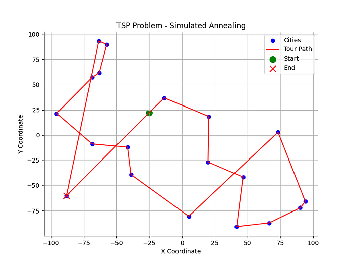

. This shows the improvement made by Simulated Annealing over the Nearest Neighbor heuristic.

Why Is This Approach Useful?

• Fast Approximation: Nearest Neighbor quickly finds a reasonable route.
• Further Optimization: Simulated Annealing refines the solution, reducing travel distance significantly.
• Practical Applications: Used in route optimization, delivery logistics, and manufacturing scheduling.
• Scalability: Although exact algorithms are infeasible for large-scale problems, this heuristic method provides a good solution within a reasonable time.

Potential Improvements

• Implement Genetic Algorithms or Ant Colony Optimization for better results.
• Introduce Tabu Search to avoid revisiting previously tested solutions.
• Use Parallel Processing to speed up execution.

This implementation demonstrates TSP approximation using heuristic and metaheuristic approaches, making it practical for real-world applications like logistics and transportation planning.